 office (412)
9679367
office (412)
96793672.3 Bond Prices: Multi-Period Case
|
T |
Cash flows from most fixed-income securities extend beyond one period. The valuation of these cash flows uses two principles: that of discounting and that of value additivity. Value additivity says that you can simply add up the different discounted cash flows. The discounting principles you have learned say that you must be careful to add together only present values at the same time.
With these principles in mind, it is easy to move to multiple periods and to multiple cash flows. One complication that arises is that different interest rates may be used to discount cash flows at different periods. For example, you may be willing to lend money for one year at 7%, but may require a higher interest rate, say, 8% per year, to lend money for two years. The extra return would compensate you for not being able to use the money for that extra year.
The interest rate used to discount cash flows in period t, r
t , is called the spot interest rate for t periods. We will quote interest rates relative to one period (which is generally one year). That is, rt per period means that interest accrues (or is paid) at the rate of rt% per period for t periods.For example, consider a zero-coupon bond that pays its face value, F, in two years. You can value this bond given the two-year spot interest rate. The arbitrage-free price of this pure discount bond is the present value of the face amount F discounted at the two-year spot interest rate.
![]()
Example: Present Value using Spot Rates of Interest
The present value of $100 at the end of two years when two-year spot interest rates are 6% per year is:
![]()
As you can see, the only differences between a cash flow in one period and a cash flow in two periods are (1) we use the two-period interest rate, and (2) we discount the cash flows "twice." If the cash flow occurs in t periods, we use the t-period spot interest rate and discount the cash flow for t periods.
With many periods, however, you can also receive intermediate payments. For example, a coupon bond makes a payment every period in addition to the face value, which is paid at maturity.
These more complex cash flows can also be valued using what you have learned in Chapter 1. First, you know how to discount each cash flow. Second, you know that you can add up the discounted cash flows, as in the derivation of the derivation of the annuity formula (see appendix A, in chapter 1).
For example, consider the timeline in Figure 2.1 for a newly issued 30-year Treasury bond with a face value of $10,000 and a coupon rate equal to 10% compounded semiannually.
|
Figure 2.1 30-Year Coupon Bond |
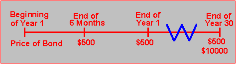
Here, we know the present value of each cash flow. Value additivity says that the value of the bond must equal the sum of all the present values, so we also know the value of the bond.
There is another way to see why value additivity must hold, and this comes from arbitrage. The cash flows from the 30-year Treasury bond are exactly the same as a portfolio of 59 zero-coupon bonds with face values equal to $500 plus one zero-coupon bond with a face value equal to $10,500. The first zero-coupon bond has maturity equal to 6 months, the second 12 months, and so on.
Since it is possible to reconstruct the Treasury bond from the zero-coupon bonds, the value of the Treasury bond must equal the value of the collection (or portfolio) of zero-coupon bonds. If the Treasury bond had a higher price, you would sell it and buy all the necessary zero-coupon bonds, giving you a pure arbitrage profit.
You can calculate the value of this bond using the procedure in Chapter 1, in the Time Value of Money topic 1.2. You should be able to verify that if the interest rate is 7%, the value of the bond is $13,741.71.
Example: Coupon Bond
Suppose you want to value a 10-year U.S. Treasury bond with a face value of $10,000 and a coupon rate equal to 6% payable semiannually. The bond is issued today.
With a face value of $10,000 and a coupon rate equal to 6% per year, the bond will pay $300 ( = 10,000 x 0.06 x 1/2 ) every six months for ten years and then pay the face value of $10,000 at the end of ten years. The cash flows are shown in the time-line in Figure 2.2.
|
Figure 2.2 10-Year Coupon Bond |
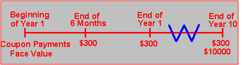
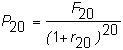
In other words, the holder of this bond receives 20 separate cash payments of $300 each and one cash payment of $10,000 over the ten years. The arbitrage-free price of each coupon payment (denoted by C = $300 for the tth coupon payment) is:
![]()
The arbitrage-free price of the face value is:
Value additivity (or lack of arbitrage) then says that the price of this bond is:
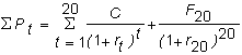
in the above each r
t is the six-month interest rate.The stream of coupon payments makes up an ordinary annuity, so the value of the bond equals the value of an ordinary annuity plus the present value of the face value.
However, you cannot apply the annuity formula directly because it assumes that all the spot interest rates are the same. In Chapter 3, (see Overview (Topic 3.1)), you will see how to value bonds when interest rates for maturities differ.
For now, if we make the simplifying assumption that all interest rates are constant, we can apply the annuity formula. You can use the software in Bond Tutor to calculate the value of any annuity.
Example: Present Value of a Coupon Bond
Assume for the bond in Figure 2.2 that each spot interest rate is 6%. What is the value of this coupon bond?
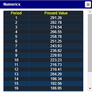
To compute this value you calculate the present value of the coupon payments and add to this number the present value of the bond’s face value. The coupon payments form an ordinary annuity. Using Bond Tutor, you can calculate that the present value of $1 for ten periods at 6% compounded twice per period is 14.8775:
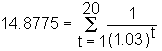
The present value of all future coupon payments for this bond (to the nearest dollar) is then:
$4,463 = $300 x 14.8775
The present value of $1 at the end of 20 periods at 3% per period is $0.5537, which is computed as follows:
![]()
Thus, the present value of the face amount is:
$5,537 = $10,000 x 0.5537
As a result, the value of the bond is $10,000. Note that this equals the face value. If a bond’s price equals its face value, it is said to be trading "at par." Otherwise, it may trade at a "discount from par" or at a "premium to par."
What happens if the market interest rate falls below or rises above 6%?
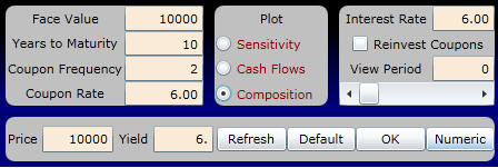
In the Bond Tutor subject two titled, Bond Values and Interest Rates, you can see what happens in each of these cases. For example, suppose we want to see how the value of the bond is altered when exposed to a range of interest rates from 1% to 10%, with a step size of 1%.
In the interactive calculator below, enter the following values:
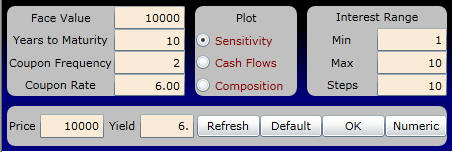
You want to look at a sensitivity analysis in step sizes of 1% (i.e., 10 steps between 1% to 10%). The exposure profile is the following:
Click on numeric button and verify the following bond values:
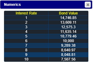
You can see that the bond value declines as interest rates increase. When the interest rate equals the coupon rate, the value equals the face amount of $10,000.
You can also see the principle of value additivity at work, by selecting to plot Cash Flows
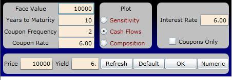
and viewing the components both numerically and graphically. For example, for the first ten coupon payments, the present value of each component is:
To see the relative weighting of coupon versus face value, click on the Composition button to view Period 0 (i.e., present time) :
The display appears as follows:
The numbers supporting the above graph for Time 0 are:
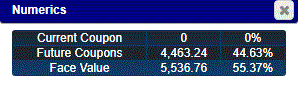
That is, the present value of the face value is $5,536.76 and the present value of the future coupon payments is $4,463.24.
The valuation principles developed thus far apply to any point in time. In the next topic, we calculate the future value of a fixed-income security.