 office (412)
9679367
office (412)
96793676.2 Cash Matching
|
C |
onceptually, the cash-matching approach to hedging is the most straightforward and provides the most control over interest rate risk. Operationally, however, it is costly and complex to implement. However, it is an interesting application of arbitrage principles, and it also provides the benchmark for comparing other approaches.
Cash matching is conceptually straightforward because any portfolio of fixed-income securities can be represented on a timeline as some sequence of cash flows, as in Figure 6.1.
Figure 6.1
Cash Flow Timeline
Cash matching merely constructs the closest synthetic equivalent to the investment using the closest available zero-coupon bonds. That is, the cash flows are replicated using a portfolio of zero-coupon bonds whose maturities coincide with each period and whose face values equal the cash flow for each maturity date. If the matching is perfect, the two positions are effectively identical.
Recall the Treasury strips example, in Chapter 4, Topic 4.7, Strips), where a the underlying position is a T-note (11 5/8% maturing on November 15, 1994) with a face value equal to $100,000. This information is presented in Figure 6.2.
Figure 6.2
Treasury Strip Cash Flows
When we calculated the value of this bond, we first replicated its cash flows using a portfolio of zero-coupon bonds. The replication is actually what is known as cash matching. In this example, the position is cash matched using a portfolio of 58.125 May 94 ci Strips, 58.125 Nov 94 ci Strips, and 1,000 Nov 94 np Strips relative to a face value of $100.
Suppose you construct the perfectly hedged portfolio that consists of long one Treasury note maturing on November 15, 1994, and short one strip portfolio (i.e., synthetic Treasury note). From the calculations provided in Chapter 4, Topic 4.8, Arbitrage Trading Strategies and Strips, the value of this hedged portfolio is:
Buying the Treasury note will cost you:
$103,968.75 + $4,972.90 = $108,941.65
Selling the synthetic Treasury note will generate:
58.125(99.75) + 1058.125(97.46875) = $108,932.10
Therefore, the value of this hedged portfolio is -$9.55. That is, it costs you slightly more to buy and sell the same cash flows than to do nothing. This is equivalent to there being no arbitrage opportunity (especially because we have not taken into account transaction costs) in the strip market.
It is also clear that the hedged position’s value is independent of shifts in the yield curve by construction because the timing and magnitude of each cash flow is covered. But consider this problem from the perspective of forward rate shifts in the yield curve. In this case, the possible set of yield curve movements that affect the market value of this position is completely described from one forward rate.
Recall that in the two-period case the relationships between the forward and the spot rates of interest are as shown in Figure 6.3.
Figure 6.3
Spot and Forward Rates of Interest
In this case, the spot two-year interest rate equals the geometric average of the Year 1 spot rate plus the forward rate for Year 1:
![]()
No matter how the forward rate of interest is ultimately realized, the value of each component in the hedged position changes precisely in the same offsetting way. This is because the net cash flows are zero.
Cash Matching Online: Example 6.2.1
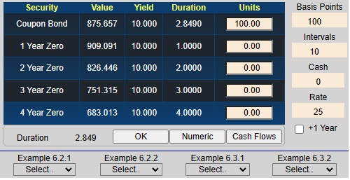
Online, consider the following position. Suppose you have 100 units of Security 1 which is a 3-year coupon bond that makes annual coupon payments equal to 5% of $1,000. In addition, suppose you have 0 units of four zero-coupon bonds with maturities ranging from 1 - 4 years. In the Duration subject of Bond Tutor, if not already shown, select "Set Position" under Example 6.2.1.
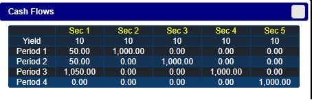
Click on the "Cash Flows" button and you should see the following window.
In the above grid you should verify that column 2,
titled Sec 1, is equivalent to a 3-year coupon bond that makes annual coupon
payments of 5% relative to a face value equal to $1000. Column 3, titled Sec 2, is equivalent to a
1-year zero coupon bond with face value equal to $1,000.
Similarly for Sec 3 (2-year zero coupon bond) and Sec 4 (three
year zero coupon bond). Next observe from this grid you can create the synthetic (i.e., cash matched) equivalent of
20 units of the coupon bond from a position of 1 Security 2 + 1 Security 3 + 21 Security 4
which is equivalent to 20 coupon bonds (Security 1). In this example, your original position is long 100 coupon bond
(i.e., 100 Sec 1 above). This position benefits from a decrease in interest rates and is
hurt by an increase in rates. If the position (shown under the "Units" column under the chart, is not already set to 100,
select "Set Position" under Example 6.2.1, or simply type 100 in the cell below 'Units' for Security 1 and
hit enter.
- Click to show/hide what your position should show.
- Click to show/hide the interest rate exposure.
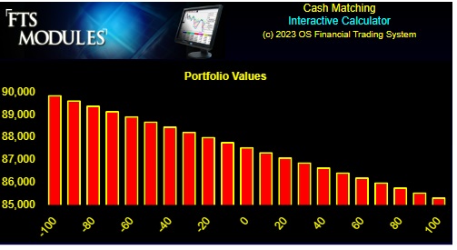
In this example, your original position is long 100 coupon bonds. This position benefits from a decrease in interest rates and is hurt from an increase in rates. The above graph reflects this decreasing position value (Y-axis) as rates increase (X-axis).
Next you can verify that the cash matching solution works by entering the offsetting synthetic position directly into the cells corresponding to units (i.e., -5 Security 2, -5 Security 3 and -105 Security 3, or alternatively, selecting "Cash Match" under Example 6.2.1 to get:
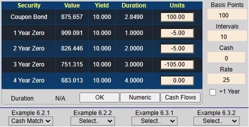
Now the position is completely hedged against interest rate risk and appears as the horizontal line as follows:
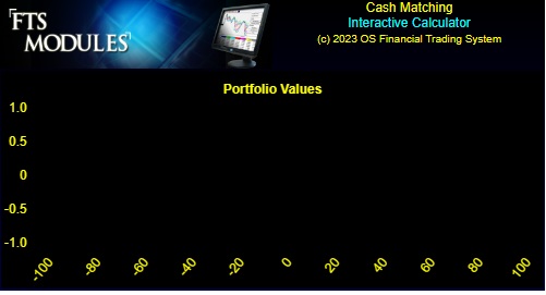
That is, the net value of the position and its synthetic opposite equals zero.
Altering Your Exposure Profile: Example 6.2.2
In general, you do not want to eliminate all risk but instead alter your exposure profile to some preferred profile. For example, suppose you predict that yield curve volatility is likely to reduce such that the yield curve will remain around the current rates. Online, you can explore different exposure profiles to find profiles that best meet your predictions.
In the following calculator, select "Set Position" under Example 6.2.2:
In the position illustrated above, a shift in either direction decreases this position's value, but you gain if the yield curve remains constant.
By changing the units you hold of each security, you can experiment with creating different exposure profiles, those that benefit from a rise in rates, those that benefit from a fall in rates, and so on.
Summary
Cash matching works because it hedges every possible dimension for a shift in the yield curve. That is, if there are 50 different cash flow dates, then there are 49 possible forward rate changes that can result in new yield curves that affect the value of the underlying position. The complexity of applying cash matching should be obvious. To hedge a large underlying position, cash matching is an immense undertaking.
At the other end of the spectrum is the concept of duration, which reduces the problem of hedging interest rate risk to one dimension. The value and limitations of duration are underscored by the important bond immunization theorem developed in the next topic.
The advantage of managing interest rate risk using duration is simplicity (and thus lower transaction costs), because only one number needs to be managed and the hedge is easily constructed. The disadvantage of this approach is that reducing the problem to one dimension means that it provides an approximation. That is, it rests upon the underlying assumptions of the bond immunization theorem.
In the next topic, you will see how you can apply Cash Matching to a zero coupon bond problem.